US4650292A - Analytic function optical component - Google Patents
Analytic function optical component Download PDFInfo
- Publication number
- US4650292A US4650292A US06/566,311 US56631183A US4650292A US 4650292 A US4650292 A US 4650292A US 56631183 A US56631183 A US 56631183A US 4650292 A US4650292 A US 4650292A
- Authority
- US
- United States
- Prior art keywords
- sub
- sup
- elements
- component
- optical
- Prior art date
- Legal status (The legal status is an assumption and is not a legal conclusion. Google has not performed a legal analysis and makes no representation as to the accuracy of the status listed.)
- Expired - Lifetime
Links
Images

Classifications
-
- G—PHYSICS
- G02—OPTICS
- G02B—OPTICAL ELEMENTS, SYSTEMS OR APPARATUS
- G02B3/00—Simple or compound lenses
- G02B3/0081—Simple or compound lenses having one or more elements with analytic function to create variable power
Definitions
- This invention in general relates to optical systems which are particularly suitable for use in cameras and, in particular, to optical elements having preferred shapes in the form of analytic functions which permit their rotation about one or more decentered pivots to maintain the focal setting of a photographic objective over a large range of object distances.
- Still another form of focusing involves the use of liquid filled flexible cells which with changing pressure can be made to perform weak dioptric tasks such as focusing.
- the changes in sagittae associated with dioptric focusing of hand camera objectives are very small, whether positive or negative, and for the usual focal lengths can be measured in but a few dozens of micrometers. It is necessary, however, that the deformed flexible cell provide sufficiently smooth optical surfaces for acceptable image quality after focusing has been performed.
- the refractive action of the sliding element when combined with the refractive action of a fixed, opposed optical surface on a nearby fixed optical element, which opposed surface is shaped in accordance with a preferred analytic function, can be made to simulate the dioptric action of a well-corrected rotational lens element of variable power.
- the invention comprises the optical elements and systems possessing the construction, combination and arrangement of elements which are exemplified in the following detailed description.
- This invention in general relates to optical systems which are particularly suitable for use in photographic cameras and, in particular, to optical elements that are shaped in accordance with preferred analytic functions or preferred polynomials which permit the elements to be relatively rotated about one or more pivots decentered with respect to an optical axis to simulate the dioptric and aspheric action of a well-corrected rotational lens element of variable power which can be used to maintain focal setting over a large range of object distances or for more complex tasks.
- the optical elements can be used singly with mirror images of themselves, or in pairs, or they can be incorporated in more elaborate systems to provide focusing action.
- the general shape of the analytic function surfaces can be represented by preferred truncated polynomial equations in two independent variables having the general form given by: ##EQU1## where i refers to surface numbers, A ijk represent coefficients, and x, y, and z refer to coordinates in a preferred non-Cartesian coordinate system.
- the novel element typically is a transparent element, preferably molded of a suitable optical plastic.
- a first surface that has a predetermined shape which is at least a part of a surface of revolution which for precision systems is preferably plano and on the other side a second aspheric surface that is asymmetric and can be described mathematically by a preselected polynomial equation having at least one nonzero term of at least fourth degree.
- the first and second surfaces of the elements are structured so that the element can be displaced generally laterally relative to the optical axis by rotation of the element about an axis of revolution, other than the optical axis, such that the second element surface operates to continuously change certain optical performance characteristics as the element moves relative to the optical axis while the first element surface remains optically invariant, not effecting any changes in any optical performance characteristics, as the element moves relative to the optical axis.
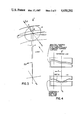
- FIG. 1 is a diagrammatic perspective view of an optical element of the invention showing its general features
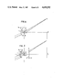
- FIG. 2 is a diagrammatic perspective view showing a pair of optical elements of the invention
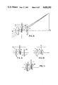
- FIG. 3 is a perspective view illustrating coordinate systems used in describing the novel surfaces of the optical elements of the invention.
- FIG. 4 is a diagrammatic cross-sectional view illustrating on the right a pair of elements of the invention and on the left a pair of rotationally symmetric dioptric elements which are simulated by the inventive elements;
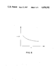
- FIG. 5 is a diagrammatic plot of certain system related parameters.
- FIGS. 6-11 are diagrammatic plan views of optical systems embodying the present invention.
- this invention generally relates to optical systems particularly suitable for use in cameras, and, more specifically, to optical elements having preferred shapes, defined in form by preferred polynomials or more generally by preferred analytic functions.
- These novel elements are unlike the prior art transversely slideable elements because their preferred analytic function surfaces permit them to be rotated about pivots decentered with respect to an optical axis to maintain focal setting or to perform more elaborate functions over a large range of object distances.
- FIG. 1 shows in diagrammatic fashion an element 10 having the general characteristics representative of the invention.
- the element 10 is a thin, transparent annular segment that can be mounted with any suitable mechanical means for rotation about an axis, RA, which is parallel to and offset with respect to an optical axis, OA.
- RA an axis
- OA optical axis
- a nominally circular area 12 which may be taken to be an aperture of maximum diameter in a designated plane in which the element 10 more or less resides.
- bundles of rays pass through the element 10 when traveling from object to image space.
- a section 14 of constant radial width that can be selectively moved into optical alignment with transmission area 12 by rotation of element 10 about the rotation axis, RA.
- One surface (16) of the peripheral section 14, as shown here, is planar and as such produces no change in its optical effect across the transmission area 12 as element 10 rotates.
- Opposing the surface 16 is another surface, 18, shown in exaggerated fashion and facing out of the paper.
- the surface 18 is distorted in the shape of a preferred analytic function that is selected according to the teaching of the invention such that useful optical changes are effected by the surface 18 as the element 10 rotates about the rotation axis, RA. It is the shape of the surface 18, or similar surfaces, that is the crux of the invention.
- an analytic function surface such as that of 18 allows an element such as 10 to be used with other closely spaced similar elements to simulate rotationally symmetric dioptric or aspheric elements of variable power.
- such elements when used in combination, can be used with one or more fixed in place and others rotating or all rotating about the same or different axes whether in the same or in opposite directions to accomplish the tasks of simulation.
- FIG. 2 diagrammatically illustrates a pair of such elements, designated at 20 and 22, adapted to oppositely rotate about the displaced axis of rotation, RA.
- Such elements can also be incorporated in more elaborate systems as the examples to follow will illustrate.
- FIG. 3 illustrates the various coordinate systems found useful in analyzing, defining and specifying the analytic function surfaces of the optical elements of the invention.
- the first one most convenient for facilitating manufacturing, is a cylindrical coordinate system arranged in a transverse plane for the treatment of the analytic surface mathematically such that the origin of coordinates in the x-y plane lies at the displaced assignable pivot point, the intersection of the rotation axis, RA, with the x-y plane.
- the rotation axis, RA, through the pivot point is taken to be parallel to the optical axis, OA, and hence the geometry in the transverse reference plane is of polar form and the analytic shape can be defined in principle in terms of ordinary polar coordinates.
- the coordinates of a point, P, on the analytic surface in the transverse plane are given by the coordinates r and phi.
- a preferred shape in three-dimensional space in the polar system is completely defined with the sagittal depth, z, or departure from the transverse plane expressed as functions of the polar coordinates in the transverse plane.
- the first of these is the x-y-z system normally employed in the course of optical design, whereby the optical axis, OA, is taken to be the z-axis, the y-z plane is taken to be the meridional plane and the x-axis, as the skew axis, is perpendicular to either.
- the values of z are positive toward the observer
- the values of y are positive upwards in the meridional plane
- the values of x are positive to the right.
- auxiliary non-Cartesian frame of reference such that its origin of coordinates, as for the x-y-z system, lies on the optical axis, OA, at the point of intersection of the optical axis, OA, with the transverse reference (x-y) plane.
- the respective origins in the two systems may be related by a translational shift along the z-axis.
- the new non-Cartesian frame of reference is related approximately to the x-y-z system but of itself involves arcs and radial extensions in the polar system.
- distances along any radius from the pivot point below in FIG. 3, less the assigned radial distance from the pivot point below to the origin of coordinates (o,o,o) become the newly defined values of y.
- Positive y-values are to the top of the origin of coordinates.
- the lengths of arcs concentric about the pivot point, as measured along the arcs from the y-axis, become the newly defined values of x, and are positive to the left, although still arcs.
- the quantity z is either the same as z, or different only by a translational constant along the z-axis.
- each has a transmitting area in the form of a sectorized annulus (see FIG. 2), and likely it is necessary for one to introduce a fixed circular defining aperture nearby as, for example, the circle 19 in Fig. 2.
- focusing or other optical action takes place when one of the two analytic shapes is rotated about the displaced pivot point, or points where two displaced axes of rotation are used, with respect to the other, or both with respect to the fixed circular aperture centered on the optical axis, OA, nearby. That is to say, in a more general case where both elements are rotatory, one may have a pivot point below for one element, as in FIG. 1, and a pivot point above for the other element (not shown), or both pivot points together but above or below, and similarly for other azimuths.
- the differential geometry of the individual analytic shape can thus begin at the intersection of the optical axis, OA, with the analytic function surface, which is the adopted origin of coordinates, and owing to the complexities of any possibly closed analytic function, can instead be conveniently described by a power series in x and y. Furthermore, total exactness of representation is not required and therefore the power series may be truncated to polynomial forms. As long as no pole or poles lie within the useful area of the sectorized annulus, there will be no mathematical singularity to deter, particularly because the inner bound is comprised of a concentric arc about the offending singularity at the pivot point.
- analytic function defining the shape of the deformed surface can be expressed in terms of a truncated power series or polynomial form to any desired precision as long as the function remains analytic within the useful aperture and as long as sufficient terms are used.
- an important goal of the invention which is the simulation of the optical action of a closely adjacent pair of rotational dioptric elements (see FIG. 4 on the left) with possible aspheric powers amongst the four surfaces, by the substitution of a closely adjacent pair of dioptric elements of analytic function form as shown on the right in FIG. 4.
- One of the simulating pair is to be rotatory about an eccentric pivot and have an outlying surface which is plane, the other which may be fixed has an outlying surface which may be of a rotational dioptric form with or without aspheric powers.
- Both these elements have inner opposed surfaces that are to take on the forms of analytic surfaces, and thereby perform the same optical action as the pair to be simulated, as nearly as possible. Furthermore, if for any given set of object distances, one finds a corresponding set of such closely adjacent rotational dioptric elements, optimized as may be desired for optical performance of an objective over the aperture, field and spectrum, the rotational dioptric elements varying not only in dioptric power but also in aspheric powers, distributed over their four surfaces in a preferred way, one must then substitute a rotatory motion of at least one of the inventive optical elements about a displaced pivot point and about an axis through the pivot point parallel to the optical axis, OA in order to vary both the equivalent dioptric and aspheric powers in simulation, as far as possible, of the optical action of the first set.
- the coefficients of the power terms must be evaluated for both the rotatory and fixed surfaces that will assist in optimizing the simulation.
- the target values of the first dioptric set to be simulated must be determined by the usual practices of optical design. The evaluation of the simulation, however, must proceed along mathematical lines.
- a first step is to carry through a detailed optical design of the desired system to be simulated for an adopted mean object distance, either central within the focusing range or decentered within the range to favor distant scenic photographs, or more rarely, to favor close-ups, according to the usage of a camera.
- This detailed design must be planned in advance, however, to incorporate at least one pair of adjacent surfaces intended to be ultimately of polynomial or analytic form, or at least inserted mathematically. If only one surface of the simulating pair is to be rotatable about a displaced axis, the simple element of which it is either the forward or rear surface must be at the start of plane form for its other surface, or else the polynomial form can be apportioned between the two sides.
- the rotatable surface is to become of analytic or polynomial form.
- the overall optical design may include, if found desirable, dioptric and aspheric powers on either or both of the inner-lying, opposed surfaces that are to become of analytic or polynomial form, and the outlying surface of the fixed element may have dioptric and aspheric powers, as may be required.
- the enjoyingle dioptric surface of the rotatable element may be transferred or apportioned onto the outlying surface of the fixed element which surface may already have predetermined dioptric and aspheric powers.
- Ths reference line will not be identical to any actual transmitted ray of light except at the optical axis, but is only a mathematical convenience in that any point on this line has the same values for x and y, varying only in z.
- An actual ray of light would instead be refracted by the successive surfaces of the adjacent simulating element pair, the inner opposed surfaces of which are to become deformed in a preferred way. While one might indeed use an actual ray of light as a reference, x and y would vary along the line segments between successive surfaces. Any power series development in x, y and z would have coefficients of considerable and probably unnecessary complexity.
- the reference line parallel to the axis and to calculate for the basic dioptric elements (on the left in FIG. 4) the total optical thickness along this reference line between the point of intercept on the first of the relevant four surfaces and the point of intercept on the last of the four surfaces.
- the optical thickness will in general consist of three line segments, two of which are in the media and the central one in air.
- the optical thickness along the reference line is the simple summation of the geometrical line-segments multiplied by the respective index of refraction.
- optical thickness as a function of x and y, calculated analytically for the dioptric basic system in which both elements are of rotational form about the optical axis, OA, that is to be reproduced by the summation of the geometrical line-segments along the same reference line, multiplied by the respective indices of refraction, where the inner-lying paired dioptric surfaces of the elements on the left in FIG. 4 are to be replaced by polynomial or more generally by analytic shapes.
- the line segment in air that is, the central segment
- the line segment in air must have the same geometrical length when the polynomial shapes are employed as when the basic rotational dioptric elements are used. All that happens is that the location of this air segment in z along the reference line shifts, but in such a way that an increased thickness along the reference line for one element is off-set by a decreased thickness for the other.
- the total optical thickness along the reference line is thus unchanged between the value for the basic or mean dioptric system to be simulated, and the substituted polynomial or analytic system in null or unrotated position that in principle simulates the basic dioptric system.
- the new aberrations are also small, being primarily a slight side-stepping of the ray of light being refracted otherwise this way and that through the optical system.
- refractive errors caused by the prismatic differential changes along any given ray from slope errors at the points of intercept, as compared to the slopes of the basic dioptric surfaces to be simulated.
- These added-on aberrations in the polynomial or simulating system are relatively small for objectives of normal aperture, field and spectral coverage as for hand camera applications, and become important only for larger systems or for systems intended for the highest acuity.
- there are additional small aberrations caused by imperfections in the simulation between the analytic representation of the deformed surfaces and the rotational dioptric surfaces of the basic system to be simulated, caused principally by truncation of the power series representations.
- the power series in x, y and z space can be cast into polar representation in r and phi.
- the externally located pole in its multiple orders indicated by the transformation terms in reciprocals of (a+y) and reciprocal powers of (a+y) now are swallowed up in such a way that the coefficients in the r and phi polar system no longer contain poles.
- the polar representation is no longer a fully complete power series, but by equivalence, at least through the order of the power series adopted, it does represent the same surface shape as obtained earlier from the analytic functions in x and y. There is no less of accuracy in the transformation to the polar system not already inherent in the bent cartesian system.
- variable quantity (a+y) appears in the denominator in various powers for a number of coefficients.
- the fact that such a term in y is variable upsets the nature of the power series in the normal representation.
- the convergence can be slow and hence one will be left with the situation that the polar representation will be somewhat more accurate than the readjusted power series truncated at an adopted level.
- This discrepancy will reappear in optimizations carried out in the x, y and z system and then transformed back again into the x, y and z system or into the polar system.
- An optimization routine carried out in the polar system presumably in the long run will yield the best results. Representation of the optimum functional shape in the polar system will then contain no poles and will be accurate in accordance with the number of terms employed.
- the appearance of ⁇ in the denominator means that the designer can use a small value of ⁇ thereby one can determine a relatively strongly deformed polynomial surface, or can use a larger value of ⁇ for a weaker deformed surface, the latter endangering the performance because of the larger contributions of the higher order terms in powers of ⁇ .
- ⁇ and phi are in the same polar system.
- Phi as used above is a variable in polar coordinates used to define the actual stationary shape of the deformed surface in polar coordinates.
- ⁇ is the angular displacement of the pre-determined deformed shape for the movable or rotatable element.
- ⁇ is the particular value of ⁇ transforms the performance of the basic system for an assigned mean object distance to compensation in focus for movement of the object plane to some other distance, possibly to infinity.
- a further step, if desired, may be performed by a computerized optimization routine, according to the quality of performance desired.
- a computerized optimization routine may be performed by a computerized optimization routine, according to the quality of performance desired.
- an array of image points must be incorporated over the full field, inasmuch as no two images are alike, and the rotational relationships of the normal system become suppressed.
- the two patterns in aperture and field will in general lead to a much prolonged computational routine, as compared to the requirements of a purely rotational system. For convenience, therefore, the optimization may be satisfactorily performed in a mean wavelength with usually adequate precision.
- the re-introduced quantities may also include the ⁇ A i0k . Indeed, all the possible terms in a matrix in x and y may be employed, but many will be small in magnitude. The computer burden may then be great.
- a final step may be to recast the fully computer-optimized shapes in x and y back into the polar system.
- this concluding transformation use should be made of the exact relationships of the transformations, point by point, in order to avoid inaccuracies re-introduced by inexact power series representation with but a reasonable number of terms.
- the final polar representation may be of value mostly for fabrication purposes, wherein the desired clear apertures of the fixed and of the movable surfaces are clearly set forth.
- each of the analytic function surfaces of the invention to simulate the variable portion of the rotational dioptric system with one or more analytic function elements rotatable about a common pivot is given in the x, y, z coordinate system by:
- f d As a scale factor can also be adapted to include distortion over a mean part of the field (calibrated focal length for infinity object).
- the optical system will also have the usual f d of gaussian optics, where for mathematical purposes the object plane is shifted temporarily to infinity.
- f d is used for a fixed and assigned position of the image plane, and f d for the concomitant but ever changing system, while obtainable, is not actually being used in the picture-taking process.
- the first example is a pair of analytic function elements combined with an objective as shown in FIG. 6.
- the constructional data in tabular form is as follows:
- Element III with its rear surface polynomial is fixed (no rotation).
- Element IV with its forward surface polynomial rotates about an assigned displaced center with the transversely displaced axis parallel to the optical axis.
- the third example, and last in the x, y, z system, is a pair of analytic function elements combined with three elements as shown in FIG. 8. Constructional data is:
- Element II with its rear surface polynomial is fixed (no rotation).
- Element III with its forward surface polynomial rotates about an assigned displaced center with the transversely diplaced axis parallel to the optical axis.
- Non-rotational coefficients are as follows:
- Surfaces 4 and 5 are th principal polynomial surfaces and have coefficient values to be disignated.
- This example focuses from infinity to approximately 25 inches with an offset distance of 0.570 inch for rotating element II.
- the base system of FIG. 9 is focusable from infinity to approximately 26 inches with a point distance of 0.6 inches and an angular excursion of the rotatable element of approximately 50° along the arc between center points of the outlying apertures.
- the system also focuses down to approximately 26 inches, but with a pivot distance of 1.0 inch.
- FIG. 10 An example of a three element all plexiglass system is shown in FIG. 10 which has the following constructional data:
- Surfaces 4 and 5 are the polynomial surfaces, although surface 3 can also be drawn upon as a polynomial surface together with revised optimization over surfaces 3, 4 and 5 collectively.
- surface 5 contains implicitly dioptric power and corrective rotational aspheric terms as a base system, all of which are thereafter contained within and replaced by the polynomial coefficients given, as follows:
- FIG. 11 a four element focusable objective which utilizes a glass replacement pair of elements, instead of the front plexiglass element of the 7th example, to get improved correction for chromatic aberration.
- This system has constructional data as follows:
- Surfaces 6 and 7 are the polynomial surfaces, although surface 5 can also be drawn upon as a polynomial surface together with revised optimization over surfaces 5, 6 and 7 collectively.
- surface 7 contains implicitly dioptric power and corrective rotational aspheric terms as a base system, all of which are thereafter contained within and replaced by the polynomial coefficients given, as follows:
- Any element so rotated must then employ either a plane surface for its outlying surface such that the transverse rotation about the displaced parallel axis causes no perceptible change in the dioptric action of this transverse plane surface, or in special cases one may apportion the work of the analytic surface from its one original face, instead, over both of the surfaces of the element.
- the outlying surface of the fixed element may be designed as with any other outlying dioptric surface or element of the optical system, and may therefore have such rotational dioptric and aspheric powers as may prove advantageous.
- both elements of a pair rotate individually about assigned displaced pivot points and displaced parallel axes, either equally but oppositely in sense of rotation as a selected important variant, or with proportional rotations of the same or opposite sense as may be desired, or even non-linearly in dual rotations of the same or opposite sense where such control may be required. All such transversely rotated elements must therefore have either plane out-lying surfaces that rotate in their own planes without optical effect, or must have the work of the respective analytic surfaces apportioned amongst the surfaces.
Abstract
Description
z=1/2c(x.sup.2 +y.sup.2)+[β+1/8(1-e.sup.2)c.sup.3 ](x.sup.2 +y.sup.2).sup.2 +. . .
(z.sub.i+1 -z.sub.i)=1/2(c.sub.i+1 -c.sub.i)(x.sup.2 +y.sup.2)+(H.sub.i+1 -H.sub.i)(x.sup.2 +y.sup.2).sup.2 +. . .
H.sub.i =β.sub.i +1/8(1-e.sup.2)c.sup.3 i
z=K.sub.1 (xy.sup.2 +1/3x.sup.3)-K.sub.2 x.sup.3 y+K.sub.3 xy.sup.3
z=K.sub.1 (xy.sup.2 +1/3x.sup.3)-K.sub.2 x.sup.3 y+K.sub.3 xy.sup.3 +K.sub.4 x.sup.4 +K.sub.5 x.sup.2 y.sup.2
__________________________________________________________________________
Element        Separations
                        Clear
Number
     Surface
          Radii
               Plastic
                   Air  Apertures
                              Material
__________________________________________________________________________
I    1    0.1776
               0.0286   0.200 Plexi
     2    0.2707*  0.0741
                        0.185
     3    stop     0.0122
                        0.085 diaphragm
II   4    -2.284*
               0.0131   0.111 Polycarbonate
     5    plano**  0.0019
                        0.105
III  6    2.186**
               0.0131   0.103 Polycarbonate
     7    plano    0.0110
                        0.096
     8    stop     0.8230 #
                        0.083 Iris & Shutter
__________________________________________________________________________
 *Aspheric (rotational)
 **Polynomial (nonrotational)Radius given is simulated for the mean object
 distance.
 # Back focal distance (d.sub.e)
 -f.sub.d = 1.0000
 s.sub.1 (adopted mean object distance) = 20.96
 -f.sub.d /10.0
f.sub.d =0.9983 (d.sub.e held constant).
______________________________________
Beta.sub.2 =
         1.754 × 10°
                      Beta.sub.4 =
                                -1.528 × 10.sup.1
Gamma.sub.2 =
         7.031 × 10.sup.-3
                      Gamma.sub.4 =
                                -2.862 × 10.sup.-2
Delta.sub.2 =
        -1.750 × 10.sup.-7
                      Delta.sub.4 =
                                -4.491 × 10.sup.-9
______________________________________
______________________________________
A.sub.520 =
       -2.288 × 10.sup.-1
                      A.sub.620 =
                                0
A.sub.502 =
       -2.288 × 10.sup.-1
                      A.sub.602 =
                                0
A.sub.530 =
        1.861 × 10.sup.-2 /-θ
                      A.sub.630 =
                                1.861 × 10.sup.-2 /-θ
A.sub.521 =
        2.288 × 10.sup.-1
                      A.sub.621 =
                                0
A.sub.512 =
        5.584 × 10.sup.-2 /-θ
                      A.sub.612 =
                                5.584 × 10.sup.-2 /-θ
A'.sub.540 =
        1.906 × 10.sup.-2
                      A'.sub.640 =
                                0
A.sub.540 =
       -1.059 × 10.sup.-2
                      A.sub.640 =
                                0
A.sub.531 =
       -1.861 × 10.sup.-2 /-θ
                      A.sub.631 =
                               -1.861 × 10.sup.-2 /-θ
A.sub.522 =
       -2.118 × 10.sup.-2
                      A.sub.622 =
                                0
A.sub.504 =
       -1.059 × 10.sup.-2
                      A.sub.604 =
                                0
A'.sub.550 =
       -9.307 × 10.sup.-4 /-θ
                      A'.sub.650 =
                               -9.307 × 10.sup.-4 /-θ
A.sub.550 =
        1.285 × 10.sup.-3 /-θ
                      A.sub.650 =
                                1.285 × 10.sup.-3 /-θ
A'.sub.541 =
       -1.906 × 10.sup.-2
                      A'.sub.641, =
                                0
A.sub.541 =
        2.118 × 10.sup.-2
                      A.sub.641 =
                                0
A.sub.532 =
        4.282 × 10.sup.-3 /-θ
                      A.sub.632 =
                                4.282 × 10.sup.-3 /-θ
A.sub.523 =
        2.118 × 10.sup.-2
                      A.sub.623 =
                                0
A.sub.514 =
        6.423 × 10.sup.-3 /-θ
                      A.sub.614 =
                                6.423 × 10.sup.-3 /-θ
______________________________________
______________________________________
                                   Clear
Element
       Sur-             Separations
                                   Aper- Mate-
Number face   Radii     Plastic
                              Air    tures rial
______________________________________
I      1      0.1147    0.0242       0.196 Plexi
       2       0.1502*        0.0004 0.192
II     3      0.1339    0.0240       0.185 Plexi
       4      0.1747          0.0792 0.171
III    5      -0.2815*  0.0054       0.071 Poly-
       6      plano**         0.0004 0.066 car-
                                           bonate
IV     7      plano**   0.0054       0.066 Poly-
       8      plano           0.1228 0.070 car-
                                           bonate
V      9       1.0063*  0.0205       0.250 Poly-
       10     4.511           0.5565#
                                     0.257 car-
                                           bonate
______________________________________
 *Aspheric (rotational)
 #Back focal distance (d.sub.F)
 **Polynominal (nonrotational); Radii given are as simulated for the mean
 object distance.
 -f.sub.d = 1.0000
 s.sub.1 (adopted mean object distance) = 13.55
 -f.sub.d /10.1
f.sub.d =0.9987 (d.sub.F held constant)
__________________________________________________________________________
Beta.sub.2 =
      -1.412 × 10.sup.1
              Beta.sub.5 =
                    -1.736 × 10.sup.2
                            Beta.sub.9 =
                                   9.233 × 10.sup.0
Gamma.sub.2 =
      -9.123 × 10.sup.-3
              Gamma.sub.5 =
                    -1.892 × 10.sup.-2
                            Gamma.sub.9 =
                                  -9.670 × 10.sup.0
Delta.sub.2 =
      -1.892 × 10.sup.-4
              Delta.sub.5 =
                    -4.442 × 10.sup.-5
                            Delta.sub.9 =
                                  -1.695 × 10.sup.-1
__________________________________________________________________________
______________________________________
A.sub.620 =
        0             A.sub.720 =
                                0
A.sub.602 =
        0             A.sub.702 =
                                0
A.sub.630 =
        4.519 × 10.sup.-2 /-θ
                      A.sub.730 =
                                4.519 × 10.sup.-2 /-θ
A.sub.621 =
        0             A.sub.721 =
                                0
A.sub.612 =
        1.356 × 10.sup.-1 /-θ
                      A.sub.712 =
                                1.356 × 10.sup.-1 /-θ
A'.sub.640 =
        0             A'.sub.740 =
                                0
A.sub.640 =
        0             A.sub.740 =
                                0
A.sub.631 =
       -4.519 × 10.sup.-2 /-θ
                      A.sub.731 =
                               -4.519 × 10.sup.-2 /-θ
A.sub.622 =
        0             A.sub.722 =
                                0
A.sub.604 =
        0             A.sub.704 =
                                0
A'.sub.650 =
       -2.259 × 10.sup.-3 /-θ
                      A'.sub.750 =
                               -2.259 × 10.sup.-3 /-θ
A.sub.650 =
       -3.234 × 10.sup.-1 /-θ
                      A.sub.750 =
                               -3.234 × 10.sup.-1 /-θ
A'.sub.641 =
        0             A'.sub.741 =
                                0
A.sub.641 =
        0             A.sub.741 =
                                0
A.sub.632 =
       -1.078 × 10.sup.0 /-θ
                      A.sub.732 =
                               -1.078 × 10.sup.0 /-θ
A.sub.623 =
        0             A.sub.723 =
                                0
A.sub.614 =
       -1.617 × 10.sup.0 /-θ
                      A.sub.714 =
                               -1.617 × 10.sup.0 /-θ
______________________________________
______________________________________
                                   Clear
Element
       Sur-             Separations
                                   Aper- Mate-
Number face   Radii     Plastic
                              Air    tures rial
______________________________________
I      1      0.1183    0.0573       0.200 Plexi
       2       0.2227*        0.0767 0.175
II     3      -0.2675*  0.0097       0.077 Poly-
       4       plano**        0.0004 0.073 car-
                                           bonate
III    5       plano**  0.0097       0.073 Poly-
       6      plano           0.1066 0.077 car-
                                           bonate
IV     7      -2.405    0.0103       0.209 Plexi
       8      0.9195    0.0206       0.220 Poly-
       9      -1.0332*        0.5570#
                                     0.220 car-
                                           bonate
______________________________________
 *Aspheric (rotational)
 #Back focal distance (d.sub.e)
 **Polynominal (nonrotational); Radii given are as simulated for the mean
 object distance.
 -f.sub.d = 1.0000
 s.sub.1 (adopted mean object distance) = 13.61
 -f.sub.d /10.0
__________________________________________________________________________
Beta.sub.2 =
      -2.095 × 10.sup.1
              Beta.sub.3 =
                    -1.642 × 10.sup.2
                            Beta.sub.9 =
                                  -1.216 × 10.sup.1
Gamma.sub.2 =
      -4.388 × 10.sup.-1
              Gamma.sub.3 =
                     1.561 × 10.sup.-1
                            Gamma.sub.9  =
                                   7.548 × 10.sup.1
Delta.sub.2 =
      -8.500 × 10.sup.-3
              Delta.sub.3 =
                    -1.271 × 10.sup.-4
                            Delta.sub.9 =
                                   3.789 × 10.sup.0
Epsilon.sub.2 =
      -8.876 × 10.sup.-5
              Epsilon.sub.3 =
                     0      Epsilon.sub.9 =
                                   1.539 × 10.sup.-1
__________________________________________________________________________
______________________________________
A.sub.420 =
        0             A.sub.520 =
                                0
A.sub.402 =
        0             A.sub.502 =
                                0
A.sub.430 =
        4.739 × 10.sup.-2 /-θ
                      A.sub.530 =
                                4.739 × 10.sup.-2 /-θ
A.sub.421 =
        0             A.sub.521 =
                                0
A.sub.412 =
        1.422 × 10.sup.-1 /-θ
                      A.sub.512 =
                                1.422 × 10.sup.-1 /-θ
A'.sub.440 =
        0             A'.sub.540 =
                                0
A.sub.440 =
        0.743 × 10.sup.0
                      A.sub.540 =
                                0
A.sub.431 =
       -4.739 × 10.sup.-2 /-θ
                      A.sub.531 =
                               -4.739 × 10.sup.-2 /-θ
A.sub.422 =
        1.487 × 10.sup.0
                      A.sub. 522 =
                                0
A.sub.404 =
        0.743 × 10.sup.0
                      A.sub.504 =
                                0
A'.sub.450 =
       -2.370 × 10.sup.-3 /-θ
                      A'.sub.550 =
                               -2.370 × 10.sup.-3 /-θ
A.sub.450 =
       -1.487 × 10.sup.-1 /-θ
                      A.sub.550 =
                               -1.487 × 10.sup.-1 /-θ
A'.sub.441 =
        0             A'.sub.541 =
                                0
A.sub.441 =
       -1.487 × 10.sup.0
                      A.sub.541 =
                                0
A.sub.432 =
       -4.955 × 10.sup.-1 /-θ
                      A.sub.532 =
                               -4.955 × 10.sup.-1 /-θ
A.sub.423 =
       -1.487 × 10.sup.0
                      A.sub.523 =
                                0
A.sub.414 =
       -7.433 × 10.sup.-1 / -θ
                      A.sub.514 =
                               -7.433 × 10.sup.-1 /-θ
______________________________________
__________________________________________________________________________
BASE SYSTEM FOR 4th, 5th AND 6th EXAMPLES
Element         Separations
                         Clear
No.  Surface
          Radii Plastic
                    Air  Apertures
                               Material
__________________________________________________________________________
1    1    0.1498
                0.0426   0.201 Plexi
     2    0.1890*   0.0856
                         0.172
2    3    plano**
                0.0120   0.094 Plexi
     4    base**    0.0122
                         --
3    5    base**
                0.0120   0.081 Plexi
     6    -0.0235*  0.1073
                         0.084
4    7    0.05742
                0.0122   0.193 Polystyrene
     8    plano       0.6813#
                         0.200
__________________________________________________________________________
 *Rotational Aspherics
 **Nonrotational (Polynomial) according to QF number
 #Back focal distance
 -f.sub.d = 0.9843
 s.sub.1 (adopted mean object distance) = 16.76
 -f.sub.d /10.0
__________________________________________________________________________
beta.sub.2 =
       1.003 × 10.sup.1
              beta.sub.6 =
                    -1.434 × 10.sup.0
                            beta.sub.7 =
                                  2.637 × 10.sup.0
gamma.sub.2 =
      -6.781 × 10.sup.0
              gamma.sub.6 =
                    -3.274 × 10.sup.-2
                            gamma.sub.7 =
                                  1.084 × 10.sup.1
delta.sub.2 =
       1.485 × 10.sup.-3
              delta.sub.6 =
                    -1.099 × 10.sup.-4
                            delta.sub.7 =
                                  1.192 × 10.sup.-1
epsilon.sub.2 =
       1.624 × 10.sup.-5
              epsilon.sub.6 =
                    -2.970 × 10.sup.-7
                            epsilon.sub.7 =
                                  1.233 × 10.sup.-3
__________________________________________________________________________
______________________________________
4th EXAMPLE NON-ROTATIONAL COEFFICIENTS
Rotatable Surface 4
                  Fixed Surface 5
Coeffi-              Coeffi-
cient  Value         cient    Value
______________________________________
B.sub.420 =
       0.17635 × 10+00
                     B.sub.520 =
                              0.33621 × 10+00
B.sub.411 =
       0.82193 × 10-01
                     B.sub.511 =
                              0.83311 × 10-01
B.sub.402 =
       0.17116 × 10+00
                     B.sub.502 =
                              0.33073 × 10+00
B.sub.430 =
       0.96509 × 10+00
                     B.sub.530 =
                              0.97725 × 10+00
B.sub.421 =
       -0.14963 × 10+00
                     B.sub.521 =
                              -0.17296 × 10-01
B.sub.412 =
       0.14764 × 10+01
                     B.sub.512 =
                              0.15668 × 10+01
B.sub.403 =
       -0.28982 × 10+00
                     B.sub.503 =
                              -0.25311 × 10+00
B.sub.440 =
       0.84407 × 10-01
                     B.sub. 540 =
                              -0.26381 × 10+02
B.sub.431 =
       -0.14376 × 10+01
                     B.sub.531 =
                              -0.10465 × 10+01
B.sub.422 =
       -0.38025 × 10+01
                     B.sub.522 =
                              -0.56745 × 10+02
B.sub.413 =
       -0.45028 × 10+01
                     B.sub.513 =
                              -0.57384 × 10+01
B.sub.404 =
       0.14459 × 10+00
                     B.sub.504 =
                              -0.26319 × 10+02
B.sub.450 =
       -0.17390 × 10+01
                     B.sub.550 =
                              -0.66473 × 10+01
B.sub.441 =
       0.15724 × 10+02
                     B.sub.541 =
                              0.16305 × 10+02
B.sub.432 =
       -0.98287 × 10+02
                     B.sub.532 =
                              -0.10847 × 10+03
B.sub.423 =
       -0.15961 × 10+02
                     B.sub.523 =
                              -0.16436 × 10+02
B.sub.414 =
       0.74777 × 10+02
                     B.sub.514 =
                              0.50115 ×  10+02
B.sub.405 =
       0.25328 × 10+02
                     B.sub.505 =
                              0.22133 × 10+02
B.sub.460 =
       0.96561 × 10-02
                     B.sub.560 =
                              0.27799 × 10-01
B.sub.451 =
       -0.23303 × 10+00
                     B.sub.551 =
                              -0.23307 × 10+00
B.sub.442 =
       -0.12419 × 10-01
                     B.sub.542 =
                              0.42022 × 10-01
B.sub.433 =
       0.13407 × 10+00
                     B.sub.533 =
                              0.13409 × 10+00
B.sub.424 =
       0.48734 × 10-02
                     B.sub.524 =
                              0.59314 × 10-01
B.sub.415 =
       0.53554 × 10-01
                     B.sub.515 =
                              0.53576 × 10-01
B.sub.406 =
       0.99630 × 10-03
                     B.sub.506 =
                              0.19145 × 10-01
B.sub.470 =
       0.11685 × 10+00
                     B.sub.570 =
                              0.11238 × 10+00
B.sub.461 =
       0.12315 × 10+01
                     B.sub.561 =
                              0.12325 × 10+01
B.sub.452 =
       0.10226 × 10+02
                     B.sub.552 =
                              0.10245 × 10+02
B.sub.443 =
       0.15969 × 10+00
                     B.sub.543 =
                              0.15946 × 10+00
B.sub.434 =
       -0.26285 × 10+01
                     B.sub.534 =
                              -0.26229 × 10+01
B.sub.425 =
       -0.25506 × 10+00
                     B.sub.525 =
                              -0.25555 × 10+00
B.sub.416 =
       -0.27879 × 10+01
                     B.sub.516 =
                              -0.28238 × 10+01
B.sub.407 =
       -0.68930 × 10+00
                     B.sub.507 =
                              -0.70525 × 10+00
                     B.sub.580 =
                              0.12113 × 10-02
                     B.sub.562 =
                              -0.43173 × 10-04
                     B.sub.544 =
                              0.36196 × 10-03
                     B.sub.526 =
                              0.28940 × 10-03
                     B.sub.508 =
                              0.10176 × 10-03
______________________________________
______________________________________
5th EXAMPLE NON-ROTATIONAL COEFFICIENTS
Rotatable Surface 4
                  Fixed Surface 5
Coeffi-              Coeffi-
cient  Value         cient    Value
______________________________________
B.sub.420 =
       0.31745 × 10+00
                     B.sub.520 =
                              0.49309 × 10+00
B.sub.411 =
       0.19416 × 10-01
                     B.sub.511 =
                              0.20374 × 10-01
B.sub.402 =
       0.31725 × 10+00
                     B.sub.502 =
                              0.49261 × 10+00
B.sub.430 =
       0.73235 × 10+00
                     B.sub.530 =
                              0.76828 × 10+00
B.sub.421 =
       -0.82315 × 10-01
                     B.sub.521  =
                              -0.95244 × 10-01
B.sub.412 =
       0.22562 × 10+01
                     B.sub.512 =
                              0.23585 × 10+01
B.sub.403 =
       -0.37735 × 10+01
                     B.sub.503 =
                              -0.38551 × 10+00
B.sub.440 =
       -0.25889 × 10-01
                     B.sub.540 =
                              -0.26488 × 10+02
B.sub.431 =
       0.88754 × 10+00
                     B.sub.531 =
                              0.13355 × 10+01
B.sub.422 =
       -0.27066 × 10+01
                     B.sub.522 =
                              -0.55631 × 10+02
B.sub.413 =
       -0.46913 × 10+01
                     B.sub.513 =
                              -0.60622 × 10+01
B.sub.404 =
       -0.31827 × 10+00
                     B.sub.504 =
                              -0.26780 × 10+02
B.sub.450 =
       0.17938 × 10+02
                     B.sub.550 =
                              0.15100 × 10+02
B.sub.441 =
       0.63013 × 10+01
                     B.sub.541 =
                              0.63070 × 10+01
B.sub.432 =
       -0.22539 × 10+03
                     B.sub.532 =
                              -0.25300 × 10+03
B.sub.423 =
       -0.19065 × 10+01
                     B.sub.523 =
                              -0.19098 × 10+01
B.sub.414 =
       0.26757 × 10+03
                     B.sub.514 =
                              0.26215 × 10+ 03
B.sub.405 =
       -0.63023 × 10+01
                     B.sub.505 =
                              -0.62411 × 10+01
B.sub.460 =
       0.32409 × 10-02
                     B.sub.560 =
                              0.21386 × 10-01
B.sub.451 =
       -0.18306 × 10+00
                     B.sub.551 =
                              -0.18308 × 10+00
B.sub.442 =
       -0.27969 × 10-02
                     B.sub.542 =
                              0.51649 × 10-01
B.sub.433 =
       0.13301 × 10+00
                     B.sub.533 =
                              0.13301 × 10+00
B.sub.424 =
       0.92066 × 10-03
                     B.sub.524 =
                              0.55366 × 10-01
B.sub.415 =
       0.47979 × 10-01
                     B.sub.515 =
                              0.47988 × 10-01
B.sub.406 =
       0.22130 × 10-03
                     B.sub.506 =
                              0.18370 × 10-01
                     B.sub.580 =
                              0.57177 × 10-04
                     B.sub.562 =
                              0.22871 × 10-03
                     B.sub.544 =
                              0.34306 ×  10-03
                     B.sub.526 =
                              0.22871 × 10-03
                     B.sub.508 =
                              0.57177 × 10-04
______________________________________
______________________________________
6th EXAMPLE NON-ROTATIONAL COEFFICIENTS
Rotatable Surface 4
                  Fixed Surface 5
Coeffi-              Coeffi-
cient  Value         cient    Value
______________________________________
B.sub.420 =
       0.46600 × 10+00
                     B.sub.520 =
                              0.62957 × 10+00
B.sub.411 =
       0.77017 × 10-01
                     B.sub.511 =
                              0.78618 × 10-01
B.sub.402 =
       0.46026 × 10+00
                     B.sub.502 =
                              0.62204 × 10+00
B.sub.430 =
       0.11176 × 10+01
                     B.sub.530 =
                              0.11489 × 10+01
B.sub.421 =
       -0.82694 × 10-01
                     B.sub.521 =
                              -0.91447 × 10-01
B.sub.412 =
       0.24534 × 10+01
                     B.sub.512 =
                              0.25386 × 10+01
B.sub.403 =
       0.55940 × 10-01
                     B.sub.503 =
                              0.53522 × 10-01
B.sub.440 =
       0.56821 × 10-01
                     B.sub.540  =
                              0.26405 × 10+02
B.sub.431 =
       0.21750 × 10+01
                     B.sub.531 =
                              0.25840 × 10+01
B.sub.422 =
       -0.49442 × 10+01
                     B.sub.522 =
                              -0.57886 × 10+02
B.sub.413 =
       -0.69085 × 10+01
                     B.sub.513 =
                              -0.81771 × 10+01
B.sub.404 =
       -0.93669 × 10-01
                     B.sub.504 =
                              -0.26554 × 10+02
B.sub.450 =
       0.54783 × 10+01
                     B.sub.550 =
                              0.24635 × 10+01
B.sub.441 =
       0.11101 × 10+02
                     B.sub.541 =
                              0.11114 × 10+02
B.sub.432 =
       -0.18539 × 10+03
                     B.sub.532 =
                              -0.21302 × 10+03
B.sub.423 =
       -0.56624 × 10+01
                     B.sub.523 =
                              -0.56598 × 10+01
B.sub.414 =
       0.25269 × 10+03
                     B.sub.514 =
                              0.24719 ×  10+03
B.sub.405 =
       -0.12350 × 10+02
                     B.sub.505 =
                              -0.12256 × 10+02
B.sub.460 =
       0.42151 × 10-02
                     B.sub.560 =
                              0.22366 × 10-01
B.sub.451 =
       -0.18961 × 10+00
                     B.sub.551 =
                              -0.18964 × 10+00
B.sub.442 =
       -0.10823 × 10-01
                     B.sub.542 =
                              0.43619 × 10-01
B.sub.433 =
       0.13247 × 10+00
                     B.sub.533 =
                              0.13249 × 10+00
B.sub.424 =
       0.18329 × 10-02
                     B.sub.524 =
                              0.56275 × 10-01
B.sub.415 =
       0.48690 × 10-01
                     B.sub.515 =
                              0.48709 × 10-01
B.sub.406 =
       0.36013 × 10-03
                     B.sub.506 =
                              0.18510 × 10-01
                     B.sub.580 =
                              0.57177 × 10-04
                     B.sub.562 =
                              0.22871 × 10-03
                     B.sub.544 =
                              0.34306 ×  10-03
                     B.sub.526 =
                              0.22871 × 10-03
                     B.sub.508 =
                              0.57177 × 10-04
______________________________________
______________________________________
7th EXAMPLE
                                   Clear
Element
       Sur-            Separations Aper- Mate-
Number face   Radii    Medium Air    tures rial
______________________________________
I      1      0.1397   0.0485        0.200 Plexi
       2       0.1503*        0.0909 0.163
II     3      plano    0.0122        0.093 Plexi
       4      base**          0.0150 0.086
III    5      base**   0.0122        0.085 Plexi
       6      2.897           0.8006#
                                     0.092
______________________________________
 *Rotational Aspheric
 #Back focal distance
 **Nonrotational (polynomial) according to present design.
 -f.sub.d = 0.9974
 s.sub.1 (adopted mean object distance) = 13.93
 -f.sub.d /10
 Rotational coefficients are:
 beta.sub.2 = 1.928 × 10.sup.1
 gamma.sub.2 = 1.018 × 10.sup.2
 delta.sub.2 = 1.191 × 10.sup.5
 epsilon.sub.2 = 1.258 × 10.sup.5
______________________________________
Rotatable Surface Fixed Surface
Coeffi-              Coeffi-
cient  Value         cient    Value
______________________________________
B.sub.410 =
       -0.17099 × 10-01
                     B.sub.510 =
                              -0.17225 × 10-01
B.sub.401 =
       0.22753 × 10-02
                     B.sub.501 =
                              0.22097 × 10-02
B.sub.420 =
       0.16375 × 10+00
                     B.sub.520 =
                              0.93754 × 10+00
B.sub.411 =
       0.94617 × 10-01
                     B.sub.511 =
                              0.95766 × 10-01
B.sub.402 =
       0.15192 × 10+00
                     B.sub.502 =
                              0.92366 × 10+00
B.sub.430 =
       0.99257 × 10+00
                     B.sub.530 =
                              0.10052 × 10+01
B.sub.421 =
       -0.21431 × 10+00
                     B.sub.521 =
                              -0.24252 × 10+00
B.sub.412 =
       0.14404 × 10+01
                     B.sub.512 =
                              0.14626 × 10+ 01
B.sub.403 =
       -0.26486 × 10+00
                     B.sub.503 =
                              -0.26536 × 10+00
B.sub.440 =
       -0.95951 × 10-02
                     B.sub.540 =
                              -0.16220 × 10+02
B.sub.431 =
       -0.14827 × 10+01
                     B.sub.531 =
                              -0.11177 × 10+01
B.sub.422 =
       -0.19776 × 10+01
                     B.sub.522 =
                              -0.37242 × 10+02
B.sub.413 =
       -0.68388 × 10+01
                     B.sub.513 =
                              -0.58275 × 10+01
B.sub.404 =
       0.32939 × 10-01
                     B.sub.504 =
                              -0.16024 × 10+02
B.sub.450 =
       0.30359 × 10+00
                     B.sub.550 =
                              -0.48918 × 10+01
B.sub.441 =
       0.16705 × 10+02
                     B.sub.541 =
                              0.17317 × 10+02
B.sub.432 =
       -0.74565 × 10+02
                     B.sub.532 =
                              -0.85360 × 10+02
B.sub.423 =
       -0.24712 × 10+02
                     B.sub.523 =
                              -0.25217 × 10+02
B.sub.414 =
       0.63656 × 10+02
                     B.sub.514 =
                              0.37524 × 10+02
B.sub.405 =
       0.16952 × 10+02
                     B.sub.505 =
                              0.13567 × 10+02
B.sub.460 =
       0.10214 × 10-01
                     B.sub.560 =
                              0.16309 × 10+04
B.sub.451 =
       -0.24900 × 10+00
                     B.sub.551 =
                              -0.24904 × 10+00
B.sub.442 =
       -0.13165 × 10-01
                     B.sub.542 =
                              0.48277 × 10+04
B.sub.433 =
       0.14230 × 10+00
                     B.sub.533 =
                              0.14231 × 10+00
B.sub.424 =
       0.51671 × 10-02
                     B.sub.524 =
                              0.48275 × 10+04
B.sub.415 =
       0.56869 × 10-01
                     B.sub.515 =
                              0.56893 × 10-01
B.sub.406 =
       0.10566 × 10-02
                     B.sub.506 =
                              0.16295 × 10+04
B.sub.470 =
       0.12357 × 10+00
                     B.sub.570 =
                              0.11882 × 10+00
B.sub.461 =
       0.13049 × 10+01
                     B.sub.561 =
                              0.13060 × 10+01
B.sub.452 =
       0.10837 × 10+02
                     B.sub.552 =
                              0.10856 × 10+02
B.sub.443 =
       0.16926 × 10+00
                     B.sub.543 =
                              0.16902 × 10+00
B.sub.434 =
       -0.27865 × 10+01
                     B.sub.534 =
                              -0.27805 × 10+01
B.sub.425 =
       -0.27037 × 10+00
                     B.sub.525 =
                              -0.27089 × 10+00
B.sub.416 =
       -0.29553 × 10+01
                     B.sub.516 =
                              -0.29934 × 10+01
B.sub.407 =
       -0.73066 × 10+00
                     B.sub.507 =
                              -0.74757 × 10+00
B.sub.480 =
       0.12233 × 10-02
                     B.sub.580 =
                              0.45586 × 10+03
B.sub.471 =
       -0.39020 × 10-03
                     B.sub. 571 =
                              -0.39020 × 10-03
B.sub.462 =
       -0.28819 × 10-03
                     B.sub.562 =
                              0.18234 × 10+04
B.sub.543 =
       -0.77884 × 10-04
                     B.sub.553 =
                              -0.77884 × 10-04
B.sub.444 =
       0.20034 × 10-04
                     B.sub.544 =
                              0.27351 × 10+04
B.sub.435 =
       0.63118 × 10-04
                     B.sub.535 =
                              0.63118 × 10-04
B.sub.426 =
       0.64329 × 10-04
                     B.sub.526 =
                              0.18234 × 10+04
B.sub.417 =
       0.62391 × 10-04
                     B.sub.517 =
                              0.62392 × 10-04
B.sub.408 =
       0.47259 × 10-04
                     B.sub.508 =
                              0.45585 × 10+03
______________________________________
______________________________________
8th EXAMPLE
                                   Clear
Element
       Sur-            Separations Aper- Mate-
Number face   Radii    Medium Air    tures rial
______________________________________
I      1      0.1450   0.0292        0.200 SK-5
       2      0.2694          0.0048 0.192 (Glass)
II     3      0.2670   0.0152        0.188 Sty-
       4       0.1503*        0.0909 0.161 rene
III    5      plano    0.0122        0.093 Plexi
       6      base**          0.0150 0.086
IV     7      base**   0.0122        0.085 Plexi
       8      2.897           0.8006#
                                     0.092
______________________________________
 *Rotational Aspheric
 #Back focal distance
 **Nonrotational (polynominal) according to present design.
 f.sub.d = 1.0063
 s.sub.1 (adopted mean object distance) = 13.93
 -f.sub.d /10
 Rotational surface coefficients are:
 beta.sub.4 = 1.508 × 10.sup.1
 gamma.sub.4 = 1.363 × 10.sup.1
 delta.sub.4 = 1.030 × 10.sup.5
 epsilon.sub.4 = 1.046 × 10.sup.5
______________________________________
Rotatable Surface Fixed Surface
Coeffi-              Coeffi-
cient  Value         cient    Value
______________________________________
B.sub.610 =
       -0.17099 × 10-01
                     B.sub.710 =
                              -0.17225 × 10-01
B.sub.601 =
       0.22753 × 10-02
                     B.sub.701 =
                              0.22097 × 10-02
B.sub.620 =
       0.16375 × 10+00
                     B.sub.720 =
                              0.93574 × 10+00
B.sub.611 =
       0.94617 × 10-01
                     B.sub.711 =
                              0.95766 × 10-01
B.sub.602 =
       0.15192 × 10+00
                     B.sub.702 =
                              0.92366 × 10+00
B.sub.630 =
       0.99257 × 10+00
                     B.sub.730 =
                              0.10052 × 10+01
B.sub.621 =
       -0.21431 × 10+00
                     B.sub.721 =
                              -0.24252 × 10+00
B.sub.612 =
       0.14404 × 10+01
                     B.sub.712 =
                              0.14626 × 10+ 01
B.sub.603 =
       -0.26486 × 10+00
                     B.sub.703 =
                              -0.26536 × 10+00
B.sub.640 =
       -0.95951 × 10-02
                     B.sub.740 =
                              -0.16220 × 10+02
B.sub.631 =
       -0.14827 × 10+01
                     B.sub.731 =
                              -0.11177 × 10+01
B.sub.622 =
       -0.19776 × 10+01
                     B.sub.722 =
                              -0.37242 × 10+02
B.sub.613 =
       -0.68388 × 10+01
                     B.sub.713 =
                              -0.58275 × 10+01
B.sub.604 =
       0.32939 × 10-01
                     B.sub.704 =
                              -0.16024 × 10+02
B.sub.650 =
       0.30359 × 10+00
                     B.sub.750 =
                              -0.48918 × 10+01
B.sub.641 =
       0.16705 × 10+02
                     B.sub.741 =
                              0.17317 × 10+02
B.sub.632 =
       -0.74565 × 10+02
                     B.sub.732 =
                              -0.85360 × 10+02
B.sub.623 =
       -0.24712 × 10+02
                     B.sub.723 =
                              -0.25217 × 10+02
B.sub.614 =
       0.63656 × 10+02
                     B.sub.714 =
                              0.37524 × 10+02
B.sub.605 =
       0.16952 × 10+02
                     B.sub.705 =
                              0.13567 × 10+02
B.sub.660 =
       0.10214 × 10-01
                     B.sub.760 =
                              0.16309 × 10+04
B.sub.651 =
       -0.24900 × 10+00
                     B.sub.751 =
                              -0.24904 × 10+00
B.sub.642 =
       -0.13165 × 10-01
                     B.sub.742 =
                              0.48277 × 10+04
B.sub.633 =
       0.14230 × 10+00
                     B.sub.733 =
                              0.14231 × 10+00
B.sub.624 =
       0.51671 × 10-02
                     B.sub.724 =
                              0.48275 × 10+04
B.sub.615 =
       0.56869 × 10-01
                     B.sub.715 =
                              0.56893 × 10-01
B.sub.606 =
       0.10566 × 10-02
                     B.sub.706 =
                              0.16295 × 10+04
B.sub.670 =
       0.12357 × 10+00
                     B.sub.770 =
                              0.11882 × 10+00
B.sub.661 =
       0.13049 × 10+01
                     B.sub.761 =
                              0.13060 × 10+01
B.sub.652 =
       0.10837 × 10+02
                     B.sub.752 =
                              0.10856 × 10+02
B.sub.643 =
       0.16926 × 10+00
                     B.sub.743 =
                              0.16902 × 10+00
B.sub.634 =
       -0.27865 × 10+01
                     B.sub.734 =
                              -0.27805 × 10+01
B.sub.625 =
       -0.27037 × 10+00
                     B.sub.725 =
                              -0.27089 × 10+00
B.sub.616 =
       -0.29553 × 10+01
                     B.sub.216 =
                              -0.29934 × 10+01
B.sub.607 =
       -0.73066 × 10+00
                     B.sub.707 =
                              -0.74757 × 10+00
B.sub.680 =
       0.12233 × 10-02
                     B.sub.780 =
                              0.45586 × 10+03
B.sub.671 =
       -0.39020 × 10-03
                     B.sub. 771 =
                              -0.39020 × 10-03
B.sub.662 =
       -0.28819 × 10-03
                     B.sub.762 =
                              0.18234 × 10+04
B.sub.653 =
       -0.77884 × 10-04
                     B.sub.753 =
                              -0.77884 × 10-04
B.sub.644 =
       0.20034 × 10-04
                     B.sub.744 =
                              0.27351 × 10+04
B.sub.635 =
       0.63118 × 10-04
                     B.sub.735 =
                              0.63118 × 10-04
B.sub.626 =
       0.64329 × 10-04
                     B.sub.726 =
                              0.18234 × 10+04
B.sub.617 =
       0.62391 × 10-04
                     B.sub.717 =
                              0.62392 × 10-04
B.sub.608 =
       0.47259 × 10-04
                     B.sub.708 =
                              0.45585 × 10+03
______________________________________
Claims (38)
z=K.sub.1 (xy.sup.2 +1/3x.sup.3)-k.sub.2 x.sup.3 y+K.sub.3 xy.sup.3
z=K.sub.1 (xy.sup.2 +1/3x.sup.3)-K.sub.2 x.sup.3 y+K.sub.3 xy.sup.3 +K.sub.4 x.sup.4 +K.sub.5 x.sup.2 y.sup.2
z=K.sub.1 (xy.sup.2 +1/3x.sup.3)-K.sub.2 x.sup.3 y+K.sub.3 xy.sup.3
z=K.sub.1 (xy.sup.2 +1/3x.sup.3)-K.sub.2 x.sup.3 y+K.sub.3 xy.sup.3 +K.sub.4 x.sup.4 +K.sub.5 x.sup.2 y.sup.2
z=K.sub.1 (xy.sup.2 +1/3x.sup.3)-K.sub.2 x.sup.3 y+K.sub.3 xy.sup.3
z=K.sub.1 (xy.sup.2 +1/3x.sup.3)-K.sub.2 x.sup.3 y+K.sub.3 xy.sup.3 +K.sub.4 x.sup.4 +K.sub.5 x.sup.2 y.sup.2
z=K.sub.1 (xy.sup.2 +1/3x.sup.3)-K.sub.2 x.sup.3 y+K.sub.3 xy.sup.3
z=K.sub.1 (xy.sup.2 +1/3x.sup.3)-K.sub.2 x.sup.3 y+K.sub.3 xy.sup.3 +K.sub.4 x.sup.4 +K.sub.5 x.sup.2 y.sup.2
z=K.sub.1 (xy.sup.2 +1/3x.sup.3)-K.sub.2 x.sup.3 y+K.sub.3 xy.sup.3
z=K.sub.1 (xy.sup.2 +1/3x.sup.3)-K.sub.2 x.sup.3 y+K.sub.3 xy.sup.3 +K.sub.4 x.sup.4 +K.sub.5 x.sup.2 y.sup.2
z=K.sub.1 (xy.sup.2 +1/3x.sup.3)-K.sub.2 x.sup.3 y+K.sub.3 xy.sup.3
z=K.sub.1 (xy.sup.2 +1/3x.sup.3)-K.sub.2 x.sup.3 y+K.sub.3 xy.sup.3 +K.sub.4 x.sup.4 +K.sub.5 x.sup.2 y.sup.2
z=K.sub.1 (xy.sup.2 +1/3x.sup.3)-K.sub.2 x.sup.3 y+K.sub.3 xy.sup.3
z=K.sub.1 (xy.sup.2 +1/3x.sup.3)-K.sub.2 x.sup.3 y+K.sub.3 xy.sup.3 +K.sub.4 x.sup.4 +K.sub.5 x.sup.2 y.sup.2
Priority Applications (1)
| Application Number | Priority Date | Filing Date | Title |
|---|---|---|---|
| US06/566,311 US4650292A (en) | 1983-12-28 | 1983-12-28 | Analytic function optical component |
Applications Claiming Priority (1)
| Application Number | Priority Date | Filing Date | Title |
|---|---|---|---|
| US06/566,311 US4650292A (en) | 1983-12-28 | 1983-12-28 | Analytic function optical component |
Publications (1)
| Publication Number | Publication Date |
|---|---|
| US4650292A true US4650292A (en) | 1987-03-17 |
Family
ID=24262363
Family Applications (1)
| Application Number | Title | Priority Date | Filing Date |
|---|---|---|---|
| US06/566,311 Expired - Lifetime US4650292A (en) | 1983-12-28 | 1983-12-28 | Analytic function optical component |
Country Status (1)
| Country | Link |
|---|---|
| US (1) | US4650292A (en) |
Cited By (52)
| Publication number | Priority date | Publication date | Assignee | Title |
|---|---|---|---|---|
| US4805998A (en) * | 1987-11-13 | 1989-02-21 | Chen Ying T | Variable anamorphic lens system |
| EP0328930A2 (en) * | 1988-02-16 | 1989-08-23 | Polaroid Corporation | Zoom lens |
| US4925281A (en) * | 1988-02-16 | 1990-05-15 | Polaroid Corporation | Zoom lens |
| US5003532A (en) * | 1989-06-02 | 1991-03-26 | Fujitsu Limited | Multi-point conference system |
| US5424872A (en) * | 1994-04-08 | 1995-06-13 | Recon/Optical, Inc. | Retrofit line of sight stabilization apparatus and method |
| US5917656A (en) * | 1996-11-05 | 1999-06-29 | Olympus Optical Co., Ltd. | Decentered optical system |
| US5950020A (en) * | 1997-01-22 | 1999-09-07 | Polaroid Corporation | Folding photographic method and apparatus |
| US5963376A (en) * | 1996-11-27 | 1999-10-05 | Olympus Optical Co., Ltd. | Variable-magnification image-forming optical system |
| US6018423A (en) * | 1995-05-18 | 2000-01-25 | Olympus Optical Co., Ltd. | Optical system and optical apparatus |
| US6066857A (en) * | 1998-09-11 | 2000-05-23 | Robotic Vision Systems, Inc. | Variable focus optical system |
| US6098887A (en) * | 1998-09-11 | 2000-08-08 | Robotic Vision Systems, Inc. | Optical focusing device and method |
| US6104540A (en) * | 1996-11-05 | 2000-08-15 | Olympus Optical Co., Ltd. | Decentered optical system |
| US6208468B1 (en) * | 1996-06-11 | 2001-03-27 | Olympus Optical Co., Ltd. | Image-forming optical system and apparatus using the same |
| US6278558B1 (en) * | 1999-09-17 | 2001-08-21 | Rong-Seng Chang | Transverse zoom lens set |
| US6366411B1 (en) | 1995-02-28 | 2002-04-02 | Canon Kabushiki Kaisha | Reflecting type optical system |
| US6549332B2 (en) | 1996-02-15 | 2003-04-15 | Canon Kabushiki Kaisha | Reflecting optical system |
| US20030107816A1 (en) * | 2001-11-14 | 2003-06-12 | Akinari Takagi | Display optical system, image display apparatus, image taking optical system, and image taking apparatus |
| US20030173502A1 (en) * | 1995-02-03 | 2003-09-18 | Dowski Edward Raymond | Wavefront coding interference contrast imaging systems |
| US6636360B1 (en) | 1995-02-28 | 2003-10-21 | Canon Kabushiki Kaisha | Reflecting type of zoom lens |
| US20030197943A1 (en) * | 2001-11-14 | 2003-10-23 | Shoichi Yamazaki | Optical system, image display apparatus, and image taking apparatus |
| US20030225455A1 (en) * | 2000-09-15 | 2003-12-04 | Cathey Wade Thomas | Extended depth of field optics for human vision |
| US20040004766A1 (en) * | 1995-02-03 | 2004-01-08 | Dowski Edward Raymond | Wavefront coded imaging systems |
| US20040145808A1 (en) * | 1995-02-03 | 2004-07-29 | Cathey Wade Thomas | Extended depth of field optical systems |
| US20040228005A1 (en) * | 2003-03-28 | 2004-11-18 | Dowski Edward Raymond | Mechanically-adjustable optical phase filters for modifying depth of field, aberration-tolerance, anti-aliasing in optical systems |
| US6842297B2 (en) | 2001-08-31 | 2005-01-11 | Cdm Optics, Inc. | Wavefront coding optics |
| US6873733B2 (en) | 2001-01-19 | 2005-03-29 | The Regents Of The University Of Colorado | Combined wavefront coding and amplitude contrast imaging systems |
| US6911638B2 (en) | 1995-02-03 | 2005-06-28 | The Regents Of The University Of Colorado, A Body Corporate | Wavefront coding zoom lens imaging systems |
| US20050267575A1 (en) * | 2001-01-25 | 2005-12-01 | Nguyen Tuan A | Accommodating intraocular lens system with aberration-enhanced performance |
| US20070058269A1 (en) * | 2005-09-13 | 2007-03-15 | Carl Zeiss Smt Ag | Catoptric objectives and systems using catoptric objectives |
| US7253960B2 (en) | 1994-06-13 | 2007-08-07 | Canon Kabushiki Kaisha | Head-up display device with rotationally asymmetric curved surface |
| WO2007115596A1 (en) * | 2006-04-07 | 2007-10-18 | Carl Zeiss Smt Ag | Microlithography projection optical system and method for manufacturing a device |
| US20070247725A1 (en) * | 2006-03-06 | 2007-10-25 | Cdm Optics, Inc. | Zoom lens systems with wavefront coding |
| EP1932492A1 (en) | 2006-12-13 | 2008-06-18 | Akkolens International B.V. | Accommodating intraocular lens with variable correction |
| WO2008077795A2 (en) | 2006-12-22 | 2008-07-03 | Amo Groningen Bv | Accommodating intraocular lens, lens system and frame therefor |
| US7561346B1 (en) * | 2007-01-12 | 2009-07-14 | Applied Energetics, Inc | Angular shear plate |
| WO2011019283A1 (en) | 2009-08-14 | 2011-02-17 | Akkolens International B.V. | Optics with simultaneous variable correction of aberrations |
| US20110063596A1 (en) * | 2006-03-27 | 2011-03-17 | Carl Zeiss Smt Ag | Projection objective and projection exposure apparatus with negative back focus of the entry pupil |
| US20120300467A1 (en) * | 2011-05-26 | 2012-11-29 | Asia Vital Components Co., Ltd. | Optical lens and lighting device |
| WO2013001299A1 (en) | 2011-06-28 | 2013-01-03 | The Technology Partnership Plc | Optical device |
| WO2013055212A1 (en) | 2011-10-11 | 2013-04-18 | Akkolens International B.V. | Accommodating intraocular lens with optical correction surfaces |
| US9011532B2 (en) | 2009-06-26 | 2015-04-21 | Abbott Medical Optics Inc. | Accommodating intraocular lenses |
| US9039760B2 (en) | 2006-12-29 | 2015-05-26 | Abbott Medical Optics Inc. | Pre-stressed haptic for accommodating intraocular lens |
| US9198752B2 (en) | 2003-12-15 | 2015-12-01 | Abbott Medical Optics Inc. | Intraocular lens implant having posterior bendable optic |
| US9271830B2 (en) | 2002-12-05 | 2016-03-01 | Abbott Medical Optics Inc. | Accommodating intraocular lens and method of manufacture thereof |
| US9280000B2 (en) | 2010-02-17 | 2016-03-08 | Akkolens International B.V. | Adjustable chiral ophthalmic lens |
| US9504560B2 (en) | 2002-01-14 | 2016-11-29 | Abbott Medical Optics Inc. | Accommodating intraocular lens with outer support structure |
| US9603703B2 (en) | 2009-08-03 | 2017-03-28 | Abbott Medical Optics Inc. | Intraocular lens and methods for providing accommodative vision |
| US20170307860A1 (en) * | 2014-12-11 | 2017-10-26 | Carl Zeiss Ag | Objective lens for a photography or film camera and method for selective damping of specific spatial frequency ranges of the modulation transfer function of such an objective lens |
| US9814570B2 (en) | 1999-04-30 | 2017-11-14 | Abbott Medical Optics Inc. | Ophthalmic lens combinations |
| US9968441B2 (en) | 2008-03-28 | 2018-05-15 | Johnson & Johnson Surgical Vision, Inc. | Intraocular lens having a haptic that includes a cap |
| DE102016125255A1 (en) * | 2016-12-21 | 2018-06-21 | Carl Zeiss Jena Gmbh | Wavefront manipulator and optical device |
| US11707354B2 (en) | 2017-09-11 | 2023-07-25 | Amo Groningen B.V. | Methods and apparatuses to increase intraocular lenses positional stability |
Citations (10)
| Publication number | Priority date | Publication date | Assignee | Title |
|---|---|---|---|---|
| US2263509A (en) * | 1939-03-21 | 1941-11-18 | Lewis Reginald Walker | Lens and method of producing it |
| GB998191A (en) * | 1963-06-24 | 1965-07-14 | Ibm | Improvements relating to lenses and to variable optical lens systems formed of such lenses |
| US3305294A (en) * | 1964-12-03 | 1967-02-21 | Optical Res & Dev Corp | Two-element variable-power spherical lens |
| US3507565A (en) * | 1967-02-21 | 1970-04-21 | Optical Res & Dev Corp | Variable-power lens and system |
| US3583790A (en) * | 1968-11-07 | 1971-06-08 | Polaroid Corp | Variable power, analytic function, optical component in the form of a pair of laterally adjustable plates having shaped surfaces, and optical systems including such components |
| US3617116A (en) * | 1969-01-29 | 1971-11-02 | American Optical Corp | Method for producing a unitary composite ophthalmic lens |
| US3632696A (en) * | 1969-03-28 | 1972-01-04 | American Optical Corp | Method for making integral ophthalmic lens |
| US3751138A (en) * | 1972-03-16 | 1973-08-07 | Humphrey Res Ass | Variable anamorphic lens and method for constructing lens |
| US3758201A (en) * | 1971-07-15 | 1973-09-11 | American Optical Corp | Optical system for improved eye refraction |
| US3827798A (en) * | 1971-04-05 | 1974-08-06 | Optical Res & Dev Corp | Optical element of reduced thickness |
-
1983
- 1983-12-28 US US06/566,311 patent/US4650292A/en not_active Expired - Lifetime
Patent Citations (10)
| Publication number | Priority date | Publication date | Assignee | Title |
|---|---|---|---|---|
| US2263509A (en) * | 1939-03-21 | 1941-11-18 | Lewis Reginald Walker | Lens and method of producing it |
| GB998191A (en) * | 1963-06-24 | 1965-07-14 | Ibm | Improvements relating to lenses and to variable optical lens systems formed of such lenses |
| US3305294A (en) * | 1964-12-03 | 1967-02-21 | Optical Res & Dev Corp | Two-element variable-power spherical lens |
| US3507565A (en) * | 1967-02-21 | 1970-04-21 | Optical Res & Dev Corp | Variable-power lens and system |
| US3583790A (en) * | 1968-11-07 | 1971-06-08 | Polaroid Corp | Variable power, analytic function, optical component in the form of a pair of laterally adjustable plates having shaped surfaces, and optical systems including such components |
| US3617116A (en) * | 1969-01-29 | 1971-11-02 | American Optical Corp | Method for producing a unitary composite ophthalmic lens |
| US3632696A (en) * | 1969-03-28 | 1972-01-04 | American Optical Corp | Method for making integral ophthalmic lens |
| US3827798A (en) * | 1971-04-05 | 1974-08-06 | Optical Res & Dev Corp | Optical element of reduced thickness |
| US3758201A (en) * | 1971-07-15 | 1973-09-11 | American Optical Corp | Optical system for improved eye refraction |
| US3751138A (en) * | 1972-03-16 | 1973-08-07 | Humphrey Res Ass | Variable anamorphic lens and method for constructing lens |
Cited By (113)
| Publication number | Priority date | Publication date | Assignee | Title |
|---|---|---|---|---|
| US4805998A (en) * | 1987-11-13 | 1989-02-21 | Chen Ying T | Variable anamorphic lens system |
| EP0328930A2 (en) * | 1988-02-16 | 1989-08-23 | Polaroid Corporation | Zoom lens |
| US4925281A (en) * | 1988-02-16 | 1990-05-15 | Polaroid Corporation | Zoom lens |
| EP0328930A3 (en) * | 1988-02-16 | 1991-07-03 | Polaroid Corporation | Zoom lens |
| US5003532A (en) * | 1989-06-02 | 1991-03-26 | Fujitsu Limited | Multi-point conference system |
| US5424872A (en) * | 1994-04-08 | 1995-06-13 | Recon/Optical, Inc. | Retrofit line of sight stabilization apparatus and method |
| US7345822B1 (en) | 1994-06-13 | 2008-03-18 | Canon Kabushiki Kaisha | Head-up display device with curved optical surface having total reflection |
| US7355795B1 (en) | 1994-06-13 | 2008-04-08 | Canon Kabushiki Kaisha | Head-up display device with curved optical surface having total reflection |
| US20080094719A1 (en) * | 1994-06-13 | 2008-04-24 | Canon Kabushiki Kaisha | Display device |
| US20080055735A1 (en) * | 1994-06-13 | 2008-03-06 | Canon Kabushiki Kaisha | Display device |
| US7495836B2 (en) | 1994-06-13 | 2009-02-24 | Canon Kabushiki Kaisha | Display device |
| US7505207B2 (en) | 1994-06-13 | 2009-03-17 | Canon Kabushiki Kaisha | Display device |
| US7262919B1 (en) | 1994-06-13 | 2007-08-28 | Canon Kabushiki Kaisha | Head-up display device with curved optical surface having total reflection |
| US7253960B2 (en) | 1994-06-13 | 2007-08-07 | Canon Kabushiki Kaisha | Head-up display device with rotationally asymmetric curved surface |
| US7538950B2 (en) | 1994-06-13 | 2009-05-26 | Canon Kabushiki Kaisha | Display device |
| US7567385B2 (en) | 1994-06-13 | 2009-07-28 | Canon Kabushiki Kaisha | Head-up display device with curved optical surface having total reflection |
| US20070001105A1 (en) * | 1995-02-03 | 2007-01-04 | Dowski Edward R Jr | Wavefront coding interference contrast imaging systems |
| US6940649B2 (en) | 1995-02-03 | 2005-09-06 | The Regents Of The University Of Colorado | Wavefront coded imaging systems |
| US7436595B2 (en) | 1995-02-03 | 2008-10-14 | The Regents Of The University Of Colorado | Extended depth of field optical systems |
| US20030173502A1 (en) * | 1995-02-03 | 2003-09-18 | Dowski Edward Raymond | Wavefront coding interference contrast imaging systems |
| US20070076296A1 (en) * | 1995-02-03 | 2007-04-05 | Dowski Edward R Jr | Wavefront coded imaging systems |
| US7554731B2 (en) | 1995-02-03 | 2009-06-30 | Omnivision Cdm Optics, Inc. | Wavefront coded imaging systems |
| US7554732B2 (en) | 1995-02-03 | 2009-06-30 | Omnivision Cdm Optics, Inc. | Wavefront coded imaging systems |
| US20080174869A1 (en) * | 1995-02-03 | 2008-07-24 | Cdm Optics, Inc | Extended Depth Of Field Optical Systems |
| US20040004766A1 (en) * | 1995-02-03 | 2004-01-08 | Dowski Edward Raymond | Wavefront coded imaging systems |
| US20040145808A1 (en) * | 1995-02-03 | 2004-07-29 | Cathey Wade Thomas | Extended depth of field optical systems |
| US20060291058A1 (en) * | 1995-02-03 | 2006-12-28 | Dowski Edward R Jr | Wavefront coded imaging systems |
| US8004762B2 (en) | 1995-02-03 | 2011-08-23 | The Regents Of The University Of Colorado, A Body Corporate | Extended depth of field optical systems |
| US7115849B2 (en) | 1995-02-03 | 2006-10-03 | The Regents Of The University Of Colorado | Wavefront coding interference contrast imaging systems |
| US7583442B2 (en) | 1995-02-03 | 2009-09-01 | Omnivision Cdm Optics, Inc. | Extended depth of field optical systems |
| US6911638B2 (en) | 1995-02-03 | 2005-06-28 | The Regents Of The University Of Colorado, A Body Corporate | Wavefront coding zoom lens imaging systems |
| US20090109535A1 (en) * | 1995-02-03 | 2009-04-30 | Cathey Jr Wade Thomas | Extended Depth Of Field Optical Systems |
| US7732750B2 (en) | 1995-02-03 | 2010-06-08 | The Regents Of The University Of Colorado | Wavefront coding interference contrast imaging systems |
| US6366411B1 (en) | 1995-02-28 | 2002-04-02 | Canon Kabushiki Kaisha | Reflecting type optical system |
| US20020105734A1 (en) * | 1995-02-28 | 2002-08-08 | Kenichi Kimura | Reflecting type optical system |
| US6785060B2 (en) | 1995-02-28 | 2004-08-31 | Canon Kabushiki Kaisha | Reflecting type optical system |
| US6639729B2 (en) | 1995-02-28 | 2003-10-28 | Canon Kabushiki Kaisha | Reflecting type of zoom lens |
| US6636360B1 (en) | 1995-02-28 | 2003-10-21 | Canon Kabushiki Kaisha | Reflecting type of zoom lens |
| US6018423A (en) * | 1995-05-18 | 2000-01-25 | Olympus Optical Co., Ltd. | Optical system and optical apparatus |
| US6549332B2 (en) | 1996-02-15 | 2003-04-15 | Canon Kabushiki Kaisha | Reflecting optical system |
| US6208468B1 (en) * | 1996-06-11 | 2001-03-27 | Olympus Optical Co., Ltd. | Image-forming optical system and apparatus using the same |
| US6104540A (en) * | 1996-11-05 | 2000-08-15 | Olympus Optical Co., Ltd. | Decentered optical system |
| US5917656A (en) * | 1996-11-05 | 1999-06-29 | Olympus Optical Co., Ltd. | Decentered optical system |
| US5963376A (en) * | 1996-11-27 | 1999-10-05 | Olympus Optical Co., Ltd. | Variable-magnification image-forming optical system |
| US5950020A (en) * | 1997-01-22 | 1999-09-07 | Polaroid Corporation | Folding photographic method and apparatus |
| US7218448B1 (en) | 1997-03-17 | 2007-05-15 | The Regents Of The University Of Colorado | Extended depth of field optical systems |
| US6098887A (en) * | 1998-09-11 | 2000-08-08 | Robotic Vision Systems, Inc. | Optical focusing device and method |
| US6066857A (en) * | 1998-09-11 | 2000-05-23 | Robotic Vision Systems, Inc. | Variable focus optical system |
| US9814570B2 (en) | 1999-04-30 | 2017-11-14 | Abbott Medical Optics Inc. | Ophthalmic lens combinations |
| US6278558B1 (en) * | 1999-09-17 | 2001-08-21 | Rong-Seng Chang | Transverse zoom lens set |
| US7025454B2 (en) | 2000-09-15 | 2006-04-11 | The Regants Of The University Of Colorado | Extended depth of field optics for human vision |
| US20030225455A1 (en) * | 2000-09-15 | 2003-12-04 | Cathey Wade Thomas | Extended depth of field optics for human vision |
| US6873733B2 (en) | 2001-01-19 | 2005-03-29 | The Regents Of The University Of Colorado | Combined wavefront coding and amplitude contrast imaging systems |
| US20050267575A1 (en) * | 2001-01-25 | 2005-12-01 | Nguyen Tuan A | Accommodating intraocular lens system with aberration-enhanced performance |
| US8062361B2 (en) | 2001-01-25 | 2011-11-22 | Visiogen, Inc. | Accommodating intraocular lens system with aberration-enhanced performance |
| US6842297B2 (en) | 2001-08-31 | 2005-01-11 | Cdm Optics, Inc. | Wavefront coding optics |
| US20060126188A1 (en) * | 2001-11-14 | 2006-06-15 | Akinari Takagi | Display optical system, image display apparatus, imae taking optical system, and image taking apparatus |
| US20030107816A1 (en) * | 2001-11-14 | 2003-06-12 | Akinari Takagi | Display optical system, image display apparatus, image taking optical system, and image taking apparatus |
| US7446943B2 (en) | 2001-11-14 | 2008-11-04 | Canon Kabushiki Kaisha | Display optical system, image display apparatus, image taking optical system, and image taking apparatus |
| US20030197943A1 (en) * | 2001-11-14 | 2003-10-23 | Shoichi Yamazaki | Optical system, image display apparatus, and image taking apparatus |
| US7012756B2 (en) | 2001-11-14 | 2006-03-14 | Canon Kabushiki Kaisha | Display optical system, image display apparatus, image taking optical system, and image taking apparatus |
| US7019909B2 (en) | 2001-11-14 | 2006-03-28 | Canon Kabushiki Kaisha | Optical system, image display apparatus, and image taking apparatus |
| US9504560B2 (en) | 2002-01-14 | 2016-11-29 | Abbott Medical Optics Inc. | Accommodating intraocular lens with outer support structure |
| US10206773B2 (en) | 2002-12-05 | 2019-02-19 | Johnson & Johnson Surgical Vision, Inc. | Accommodating intraocular lens and method of manufacture thereof |
| US9271830B2 (en) | 2002-12-05 | 2016-03-01 | Abbott Medical Optics Inc. | Accommodating intraocular lens and method of manufacture thereof |
| US20040228005A1 (en) * | 2003-03-28 | 2004-11-18 | Dowski Edward Raymond | Mechanically-adjustable optical phase filters for modifying depth of field, aberration-tolerance, anti-aliasing in optical systems |
| US20070127041A1 (en) * | 2003-03-28 | 2007-06-07 | Dowski Edward R Jr | Mechanically-adjustable optical phase filters for modifying depth of field, aberration-tolerance, anti-aliasing in optical systems |
| US7679830B2 (en) | 2003-03-28 | 2010-03-16 | The Regents Of The University Of Colorado | Optical systems utilizing multiple phase filters to increase misfocus tolerance |
| US7180673B2 (en) | 2003-03-28 | 2007-02-20 | Cdm Optics, Inc. | Mechanically-adjustable optical phase filters for modifying depth of field, aberration-tolerance, anti-aliasing in optical systems |
| US9198752B2 (en) | 2003-12-15 | 2015-12-01 | Abbott Medical Optics Inc. | Intraocular lens implant having posterior bendable optic |
| US7719772B2 (en) | 2005-09-13 | 2010-05-18 | Carl Zeiss Smt Ag | Catoptric objectives and systems using catoptric objectives |
| US9465300B2 (en) | 2005-09-13 | 2016-10-11 | Carl Zeiss Smt Gmbh | Catoptric objectives and systems using catoptric objectives |
| US20090262443A1 (en) * | 2005-09-13 | 2009-10-22 | Carl Zeiss Smt Ag | Catoptric objectives and systems using catoptric objectives |
| US20070058269A1 (en) * | 2005-09-13 | 2007-03-15 | Carl Zeiss Smt Ag | Catoptric objectives and systems using catoptric objectives |
| WO2007031271A1 (en) * | 2005-09-13 | 2007-03-22 | Carl Zeiss Smt Ag | Microlithography projection optical system, method for manufacturing a device and method to design an optical surface |
| US20090046357A1 (en) * | 2005-09-13 | 2009-02-19 | Carl Zeiss Smt Ag | Catoptric objectives and systems using catoptric objectives |
| US7414781B2 (en) | 2005-09-13 | 2008-08-19 | Carl Zeiss Smt Ag | Catoptric objectives and systems using catoptric objectives |
| US8169694B2 (en) | 2005-09-13 | 2012-05-01 | Carl Zeiss Smt Gmbh | Catoptric objectives and systems using catoptric objectives |
| US7710658B2 (en) | 2006-03-06 | 2010-05-04 | Omnivision Cdm Optics, Inc. | Zoom lens systems with wavefront coding |
| US20070247725A1 (en) * | 2006-03-06 | 2007-10-25 | Cdm Optics, Inc. | Zoom lens systems with wavefront coding |
| US8094380B2 (en) | 2006-03-27 | 2012-01-10 | Carl Zeiss Smt Gmbh | Projection objective and projection exposure apparatus with negative back focus of the entry pupil |
| US8810927B2 (en) | 2006-03-27 | 2014-08-19 | Carl Zeiss Smt Gmbh | Projection objective and projection exposure apparatus with negative back focus of the entry pupil |
| US20110063596A1 (en) * | 2006-03-27 | 2011-03-17 | Carl Zeiss Smt Ag | Projection objective and projection exposure apparatus with negative back focus of the entry pupil |
| US20090052073A1 (en) * | 2006-04-07 | 2009-02-26 | Carl Zeiss Smt Ag | Microlithography projection optical system and method for manufacturing a device |
| CN101416117B (en) * | 2006-04-07 | 2014-11-05 | 卡尔蔡司Smt有限责任公司 | Microlithography projection optical system, tools and manufacturing method |
| US9482961B2 (en) | 2006-04-07 | 2016-11-01 | Carl Zeiss Smt Gmbh | Microlithography projection optical system, tool and method of production |
| WO2007115596A1 (en) * | 2006-04-07 | 2007-10-18 | Carl Zeiss Smt Ag | Microlithography projection optical system and method for manufacturing a device |
| US20090051890A1 (en) * | 2006-04-07 | 2009-02-26 | Carl Zeiss Smt Ag | Microlithography projection optical system, tool and method of production |
| US8970819B2 (en) | 2006-04-07 | 2015-03-03 | Carl Zeiss Smt Gmbh | Microlithography projection optical system, tool and method of production |
| US20100094413A1 (en) * | 2006-12-13 | 2010-04-15 | Akkolens International B.V. | Accommodating intraocular lens with variable correction |
| US10463473B2 (en) | 2006-12-13 | 2019-11-05 | Akkolens International B.V. | Accommodating intraocular lens with variable correction |
| EP1932492A1 (en) | 2006-12-13 | 2008-06-18 | Akkolens International B.V. | Accommodating intraocular lens with variable correction |
| US8182531B2 (en) | 2006-12-22 | 2012-05-22 | Amo Groningen B.V. | Accommodating intraocular lenses and associated systems, frames, and methods |
| US8496701B2 (en) | 2006-12-22 | 2013-07-30 | Amo Groningen B.V. | Accommodating intraocular lenses and associated systems, frames, and methods |
| US7871437B2 (en) | 2006-12-22 | 2011-01-18 | Amo Groningen B.V. | Accommodating intraocular lenses and associated systems, frames, and methods |
| WO2008077795A2 (en) | 2006-12-22 | 2008-07-03 | Amo Groningen Bv | Accommodating intraocular lens, lens system and frame therefor |
| US20110112638A1 (en) * | 2006-12-22 | 2011-05-12 | Amo Groningen Bv | Accommodating intraocular lenses and associated systems, frames, and methods |
| WO2008077795A3 (en) * | 2006-12-22 | 2010-11-25 | Amo Groningen Bv | Accommodating intraocular lens, lens system and frame therefor |
| US9039760B2 (en) | 2006-12-29 | 2015-05-26 | Abbott Medical Optics Inc. | Pre-stressed haptic for accommodating intraocular lens |
| US7561346B1 (en) * | 2007-01-12 | 2009-07-14 | Applied Energetics, Inc | Angular shear plate |
| US9968441B2 (en) | 2008-03-28 | 2018-05-15 | Johnson & Johnson Surgical Vision, Inc. | Intraocular lens having a haptic that includes a cap |
| US10052194B2 (en) | 2009-06-26 | 2018-08-21 | Johnson & Johnson Surgical Vision, Inc. | Accommodating intraocular lenses |
| US9011532B2 (en) | 2009-06-26 | 2015-04-21 | Abbott Medical Optics Inc. | Accommodating intraocular lenses |
| US9603703B2 (en) | 2009-08-03 | 2017-03-28 | Abbott Medical Optics Inc. | Intraocular lens and methods for providing accommodative vision |
| WO2011019283A1 (en) | 2009-08-14 | 2011-02-17 | Akkolens International B.V. | Optics with simultaneous variable correction of aberrations |
| US9280000B2 (en) | 2010-02-17 | 2016-03-08 | Akkolens International B.V. | Adjustable chiral ophthalmic lens |
| US20120300467A1 (en) * | 2011-05-26 | 2012-11-29 | Asia Vital Components Co., Ltd. | Optical lens and lighting device |
| WO2013001299A1 (en) | 2011-06-28 | 2013-01-03 | The Technology Partnership Plc | Optical device |
| WO2013055212A1 (en) | 2011-10-11 | 2013-04-18 | Akkolens International B.V. | Accommodating intraocular lens with optical correction surfaces |
| US20170307860A1 (en) * | 2014-12-11 | 2017-10-26 | Carl Zeiss Ag | Objective lens for a photography or film camera and method for selective damping of specific spatial frequency ranges of the modulation transfer function of such an objective lens |
| US10746975B2 (en) * | 2014-12-11 | 2020-08-18 | Carl Zeiss Ag | Objective lens for a still or film camera and method for selective damping of specific spatial frequency ranges of the modulation transfer function of such an objective lens |
| DE102016125255A1 (en) * | 2016-12-21 | 2018-06-21 | Carl Zeiss Jena Gmbh | Wavefront manipulator and optical device |
| US11707354B2 (en) | 2017-09-11 | 2023-07-25 | Amo Groningen B.V. | Methods and apparatuses to increase intraocular lenses positional stability |
Similar Documents
| Publication | Publication Date | Title |
|---|---|---|
| US4650292A (en) | Analytic function optical component | |
| Kingslake | Optical system design | |
| US4015897A (en) | Four element lens system | |
| EP3779551A1 (en) | Camera lens, camera module, and terminal | |
| CN102298197B (en) | Imaging lens, it is equipped with its optical device and the method for manufacturing imaging lens | |
| US4786153A (en) | Large-aperture macro lens system | |
| US6078411A (en) | Real-image finder optical system and apparatus using the same | |
| US4256373A (en) | Fish eye lens system | |
| US4925281A (en) | Zoom lens | |
| JPH04267212A (en) | Ultra wide angle lens | |
| CN101794014B (en) | Zoom lens, optical apparatus equipped therewith and method for manufacturing the zoom lens | |
| US4474436A (en) | Finite distance zoom lens system | |
| CN111323895A (en) | Lens and manufacturing method thereof | |
| JPS6161655B2 (en) | ||
| US4057328A (en) | Enlarging lens system | |
| CN110554478A (en) | lens and manufacturing method thereof | |
| EP0187177B1 (en) | Analytic function optical component | |
| CA1321725C (en) | Zoom lens | |
| CN110320637B (en) | Lens and method for manufacturing the same | |
| US4447135A (en) | Zoom lens system | |
| US4373786A (en) | Photographic objective of reduced size | |
| US3784277A (en) | Corrected optical system for shallow camera or the like, components thereof | |
| CA1252655A (en) | Analytic function optical component | |
| US2803997A (en) | Image-forming optical lens telephoto systems | |
| US5946145A (en) | Variable focal length optical system |
Legal Events
| Date | Code | Title | Description |
|---|---|---|---|
| AS | Assignment |
Owner name: POLAROID CORPORATION, 549 TECHNOLOGY SQUARE, CAMBR Free format text: ASSIGNMENT OF ASSIGNORS INTEREST.;ASSIGNORS:BAKER, JAMES G.;PLUMMER, WILLIAM T.;REEL/FRAME:004214/0108;SIGNING DATES FROM 19831222 TO 19831223 |
|
| STCF | Information on status: patent grant |
Free format text: PATENTED CASE |
|
| FPAY | Fee payment |
Year of fee payment: 4 |
|
| FPAY | Fee payment |
Year of fee payment: 8 |
|
| REMI | Maintenance fee reminder mailed | ||
| FPAY | Fee payment |
Year of fee payment: 12 |
|
| SULP | Surcharge for late payment | ||
| AS | Assignment |
Owner name: MORGAN GUARANTY TRUST COMPANY OF NEW YORK, NEW YOR Free format text: SECURITY AGREEMENT;ASSIGNOR:POLAROID CORPORATION;REEL/FRAME:011658/0699 Effective date: 20010321 |
|
| AS | Assignment |
Owner name: POLAROID CORPORATION (F/K/A OEP IMAGING OPERATING Free format text: U.S. BANKRUPTCY COURT DISTRICT OF DELAWARE ORDER AUTHORIZING RELEASE OF ALL LIENS;ASSIGNOR:JPMORGAN CHASE BANK, N.A. (F/K/A MORGAN GUARANTY TRUST COMPANY OF NEW YORK);REEL/FRAME:016621/0377 Effective date: 20020418 |
|
| AS | Assignment |
Owner name: OEP IMAGING OPERATING CORPORATION,NEW YORK Free format text: ASSIGNMENT OF ASSIGNORS INTEREST;ASSIGNOR:POLAROID CORPORATION;REEL/FRAME:018584/0600 Effective date: 20020731 Owner name: OEP IMAGING OPERATING CORPORATION, NEW YORK Free format text: ASSIGNMENT OF ASSIGNORS INTEREST;ASSIGNOR:POLAROID CORPORATION;REEL/FRAME:018584/0600 Effective date: 20020731 |
|
| AS | Assignment |
Owner name: POLAROID CORPORATION (FMR OEP IMAGING OPERATING CO Free format text: SUPPLEMENTAL ASSIGNMENT OF PATENTS;ASSIGNOR:PRIMARY PDC, INC. (FMR POLAROID CORPORATION);REEL/FRAME:019077/0001 Effective date: 20070122 |